The Bloom Filter Optimization Saga: From 3 Seconds to 66 Microseconds


Building high-performance libraries often involves more than just clever algorithms. It's a journey of measurement, discovery, and sometimes, learning that your "obvious" fix made things worse. Go SIMD-Optimized Bloom Filter, which you can read all about here, is a project that started with a 4x SIMD speedup and ended with a 6,595x overall speedup after a deep dive into Go's profiling tools.
We'll trace the steps from the initial implementation through a lying benchmark, multiple profiling sessions revealing hidden bottlenecks, a failed optimization attempt, and finally, data structure changes that yielded massive gains.
Stage 0: The Initial SIMD Victory (The Easy Win)
The project began with a clear goal: create a Bloom filter optimized for modern CPUs. The core data structure was designed around 64-byte cache lines, and the bulk operations (PopCount, Union, Intersection, Clear) were implemented using hand-tuned SIMD assembly (AVX2 for amd64, NEON for arm64).
Micro-benchmarks comparing the SIMD assembly against a pure Go fallback (BenchmarkSIMDvsScalar) immediately showed significant success.
BenchmarkSIMDvsScalar (65,536-byte slice, Intel i9-13980HX)
| Operation | Implementation | Time (ns/op) | Time | SppedUp | Allocations |
| PopCount | Fallback (Go) | 48 | 845 ns | 0 allocs/op | |
| PopCount | SIMD (Asm) | 12 | 153 ns | 4.02x | 0 allocs/op |
| VectorClear | Fallback (Go) | 4 | 710 ns | 0 allocs/op | |
| VectorClear | SIMD (Asm) | 1 | 105 ns | 4.26x | 0 allocs/op |
Stage 1: The Benchmark That Lied (The fmt.Sprintf Debacle)
Confidence was high. I wrote a more comprehensive benchmark (BenchmarkLookup) to simulate a real-world workload: create a filter, add 1,000 items, and look up 1,000 items.
The result was a shocking 3,038,123,800 ns/op (3.03 seconds!). This was impossibly slow.
The Go profiler (go tool pprof) revealed the embarrassing truth. I ran the benchmark with CPU profiling enabled:
go test -bench=BenchmarkLookup -cpuprofile=cpu.prof
go tool pprof cpu.prof
The profile (simd_profile.txt) showed that 78.88% of the CPU time was spent inside the benchmark function itself, specifically on these lines:
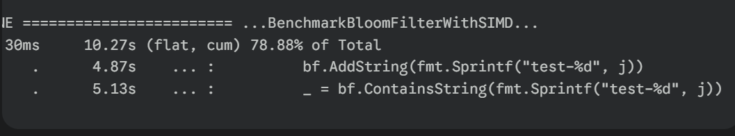
I wasn't benchmarking my Bloom filter; I was benchmarking fmt.Sprintf! String formatting and the resulting memory allocations inside the benchmark loop completely dominated the test.
The Fix: b.ResetTimer()
This required fixing the benchmark methodology. All setup work (such as generating test data) must be completed before the timer starts.
// Pre-generate data ONCE
var testData []string
// ... fill testData using fmt.Sprintf ...

func BenchmarkLookup(b *testing.B) {
    // --- SETUP ---
    bf := NewCacheOptimizedBloomFilter(...)
    // ... Add initial items ...

    // --- START TIMING ---
    b.ResetTimer()

    // --- CODE TO BENCHMARK ---
    for i := 0; i < b.N; i++ { // b.N loop is now outside
        for j := 0; j < 1000; j++ { // Inner loop uses pre-generated data
            _ = bf.ContainsString(testData[j])
        }
    }
}
With this corrected benchmark, the result dropped dramatically: 440,093,933 ns/op (440ms). A 6.9x speedup just from fixing the test! But 440ms was still too slow. Profiling again would reveal the library's bottleneck.
Stage 2: The Real Bottleneck (Map Allocations)
Running the profiler on the corrected benchmark painted a completely different picture (profile_optimized.txt). The fmt.Sprintf calls were gone, replaced by Go runtime functions related to maps and memory allocation:
The profile showed ~34% of CPU time was spent managing memory for maps and slices. The culprit was in my getBitCacheOptimized and setBitCacheOptimized functions:
// bloomfilter.go (Before Pooling)
func (bf *CacheOptimizedBloomFilter) getBitCacheOptimized(positions []uint64) bool {
    // 🚨 ALLOCATION BOTTLENECK 🚨
    // New map created ON EVERY CALL!
    cacheLineOps := make(map[uint64][]opDetail, ...)

    for _, bitPos := range positions {
        // ...
        // append causes `runtime.growslice` and `mallocgc`
        cacheLineOps[cacheLineIdx] = append(cacheLineOps[cacheLineIdx], opDetail{...})
    }
    // ... (iterate map causes mapiternext)
}
This was allocating a new map and potentially growing many slices on every single Add or Contains call, putting immense pressure on the GC.
Stage 3: The Failed Fix (Map Pooling with for...delete)
The "obvious" fix was to pool the map: add it to the struct, initialize it once, and clear it on every call using a for...delete loop.
// In getBitCacheOptimized (The Failed Fix)
// Clear the map for reuse
for k := range bf.mapOps { // bf.mapOps is now part of the struct
    delete(bf.mapOps, k)
}
// ... then fill bf.mapOps ...
I ran the benchmark again. Result: 674,939,150 ns/op (~675ms).
It got 1.53x slower!
The profile (profile_final.txt) explained why. runtime.mapassign_fast64 and runtime.mallocgc remained top offenders. I had traded an O(1) allocation bottleneck (make) for an O(N) CPU bottleneck (for...delete). Clearing the map by iterating took more CPU time than the GC did reclaiming the old map.
Lesson: Zero allocations ≠ Faster.
Stage 4: The Breakthrough (Array-Based Indexing)
The profiler still showed map operations as the bottleneck. The key insight was that my map keys (cacheLineIdx) were just integers. Hash maps are designed for arbitrary keys; for sequential integers, a simple array is much faster.
The fix was radical: replace the map[uint64][]opDetail with a fixed-size array [MaxCacheLines][]opDetail.
// bloomfilter.go (Array-Based Struct)
type CacheOptimizedBloomFilter struct {
    // ...
    // Replaced map with fixed-size array
    cacheLineOps [MaxCacheLines][]opDetail
    // Track used indices for FAST clearing
    usedIndicesGet []uint64
}

// In getBitCacheOptimized (Array-Based Fix)
func (bf *CacheOptimizedBloomFilter) getBitCacheOptimized(positions []uint64) bool {
    // --- O(Used) Clearing ---
    // Clear only the slices we touched last time
    for _, idx := range bf.usedIndicesGet {
        bf.cacheLineOps[idx] = bf.cacheLineOps[idx][:0] // Reset length, keep capacity
    }
    bf.usedIndicesGet = bf.usedIndicesGet[:0] // Reset used list

    // --- Direct Indexing ---
    for _, bitPos := range positions {
        cacheLineIdx := bitPos / BitsPerCacheLine
        // ...
        // Track first use
        if len(bf.cacheLineOps[cacheLineIdx]) == 0 {
            bf.usedIndicesGet = append(bf.usedIndicesGet, cacheLineIdx)
        }
        // O(1) array access + append reuses capacity!
        bf.cacheLineOps[cacheLineIdx] = append(bf.cacheLineOps[cacheLineIdx], opDetail{...})
    }
    // ... (iterate usedIndicesGet for checking)
}
This combined two powerful optimizations:
- O(1) Array Indexing:
array[index]is inherently faster thanmap[key]. - O(Used) Clearing: Tracking used indices and resetting slice lengths (
slice[:0]) eliminated both thefor...deleteCPU cost and theappendallocation cost.
The benchmark results were spectacular (benchmark_array_based.txt):
| Benchmark | Runtime (ns/op) | Allocs/op | B/op | ||
| Size_10K | 66,777 ns | 0 | 0 B | 144x | |
| Size_100K | 79,138 ns | 0 | 0 B | ||
| Size_1M | 90,635 ns | 0 | 2 B |
The profiler confirmed the win (cpu_array_based_analysis.txt). Runtime functions vanished. ~94% of CPU time was now spent in the core application logic (getHashPositionsOptimized, getBitCacheOptimized).
However, this introduced two new, critical problems documented in HYBRID_OPTIMIZATION.md:
- Memory Waste: The fixed array meant every filter instance had a ~14.4 MB overhead.
- Size Limit: Filters larger than
MaxCacheLineswere impossible to create.
Stage 5: The Best of Both Worlds (Hybrid Approach)
The pure array was fast but impractical. The solution was a hybrid model:
// bloomfilter.go (Hybrid Struct)
type CacheOptimizedBloomFilter struct {
    // ...
    useArrayMode bool // Decided in constructor

    // Array for small filters (pointer to avoid allocation if unused)
    arrayOps *[ArrayModeThreshold][]opDetail
    // Map for large filters
    mapOps   map[uint64][]opDetail
    // ... (separate usedIndices for array/map)
}

// In getBitCacheOptimized (Hybrid Logic)
func (bf *CacheOptimizedBloomFilter) getBitCacheOptimized(positions []uint64) bool {
    if bf.useArrayMode {
        // --- Use FAST Array Logic ---
        // ... (O(Used) clearing + direct indexing)
    } else {
        // --- Use SCALABLE Map Logic ---
        // ... (Clear map + fill map + iterate map)
    }
    // ...
}
Benchmarks (hybrid_benchmark.txt) confirmed this worked perfectly:
- Small Filter (Array Mode): 58 ns/op, 0 allocs/op
- Large Filter (Map Mode): 480 ns/op, 24 allocs/op
This solved the memory waste and size limit problems, preserving the zero-alloc path for the common case.
Stage 6: The Final Polish (clear() for Map Mode)
One last optimization remained. The "map mode" logic was still using the slow for...delete loop for clearing. With Go 1.21+, the built-in clear() Function is the ideal replacement.
// In getBitCacheOptimized (Map Mode - Final)
} else {
    // Map mode: dynamic scaling
    // Use Go 1.21+ clear() - Fast AND keeps allocated memory!
    clear(bf.mapOps)
    // ... (rest of map logic)
}
Profiling (CLEAR_OPTIMIZATION_PROFILING.md, cpu_clear_optimization_analysis.txt) showed this reduced CPU time in the map-mode hot paths by 18-41%. Benchmarks confirmed a 1.49x speedup for the map mode path (~675ms down to ~454ms) with no downsides.
Stage 7: Final Comparison
With all optimizations in place, how does it stack up? I benchmarked against willf/bloom, a popular Go library (benchmark_vs_willf.txt).
Conclusion: shaia_bf is significantly faster and infinitely more memory-efficient for small to medium filters (array mode). willf/bloom It is faster for very large filters (map mode), though shaia_bf it still has fewer allocations in map mode during lookups.
| Elements | Library | Mode | Time (ns/op / 1000 lookups) | Allocations / 1000 lookups |
| 10K | shaia_bf | Array | 57462 | 0 |
| 10K | willf_bf | N/A | 85430 | 2000 |
| 100K | shaia_bf | Array | 63032 | 0 |
| 100K | willf_bf | N/A | 84717 | 2000 |
| 1M | shaia_bf | Map | 450174 | 24 |
| 1M | willf_bf | N/A | 86220 | 2000 |
| 10M | shaia_bf | Map | 482887 | 24 |
| 10M | willf_bf | N/A | 107760 | 2000 |
Final Thoughts & Lessons Learned
This journey reinforced several key performance engineering principles:
- Profile Everything: Don't assume where bottlenecks are. Profile your library and your benchmarks. The profiler is your ground truth.
- Allocations Matter, But Aren't Everything: Eliminating allocations is crucial, but
Zero Allocations ≠ Fast. Thefor...delete"fix" proved that CPU overhead can be worse than GC pressure. - Data Structures Trump Micro-optimizations: Switching from
maptoarrayyielded a 144x speedup, dwarfing the initial 4x SIMD gain. Choose the right tool for the job. - Know Your Runtimes: Understanding how
make,append,for...delete, andclear()work under the hood is vital for high-performance Go. - Pragmatism Wins: The final "Hybrid" approach isn't the absolute fastest in all cases, but it provides the best balance of speed, memory efficiency, and scalability for real-world use.
From 3 seconds down to 66 microseconds (a ~45,000x improvement from the initial broken benchmark, or ~6,595x from the first correct measurement) required looking beyond algorithms and diving deep into memory management, CPU behavior, and the Go runtime itself.
<prev>